Busbar Analysis

Click "Open in Colab" to experiment with different parameters

Theory & Governing Equations
Simulation Results
Implementation Code

Theory

Energy Balance Equation

Q_{g e n} + / Q_{i n} - Q_{c o n v} - / W_{o u t} = \frac{d U}{d t}

Busbar Specific Variables

(I^{2} \cdot R) - (h \cdot A_{s} \cdot (T - T_{a m b})) = m \cdot C_{p} \cdot \frac{d T}{d t}

Key Equations

Equation	Formula
Heat Generation	$Q_{g e n} = I^{2} \cdot R$
Convection (Dissipation)	$Q_{c o n v} = h_{c o n v} \cdot A_{s} \cdot (T_{s u r f a c e} - T_{a m b i e n t})$
Cross-Section Area	$A = w \cdot h_{d i m}$
Surface Area (Cooling)	$A_{s} = 2 \cdot L \cdot (w + h_{d i m})$
Temp-Dependent Resistance	$R (T) = R_{r e f} \cdot [1 + α \cdot (T_{e n d} - T_{r e f})]$
Mass	$m = density \times (L \cdot w \cdot h_{d i m})$

Heat Transfer Variables

Symbol	Definition	Unit (SI)
$Q_{g e n}$	Rate of internal heat generation (Joule heating)	Watts (W)
$Q_{c o n v}$	Rate of heat loss via convection	Watts (W)
$I$	Electrical current flowing through the busbar	Amperes (A)
$R$	Electrical resistance (temp-dependent)	Ohms ( $Ω$ )
$R_{r e f}$	Resistance at the reference temperature	Ohms ( $Ω$ )
$ρ$	Electrical resistivity of the material	$Ω \cdot m$
$L$	Length of the busbar	Meters (m)
$w$	Width of the busbar	Meters (m)
$h_{d i m}$	Height of the busbar	Meters (m)
$A$	Cross-sectional area	$m^{2}$
$A_{s}$	Surface area for cooling	$m^{2}$
$h$	Convective heat transfer coefficient	$W / (m^{2} \cdot K)$
$T$	Instantaneous temperature of the busbar	$^{\circ} C$ or $K$
$T_{a m b}$	Ambient temperature of the surrounding air	$^{\circ} C$ or $K$
$T_{r e f}$	Reference temperature (usually $20^{\circ} C$ )	$^{\circ} C$ or $K$
$α$	Temperature coefficient of resistance	$1 /^{\circ} C$
$m$	Mass of the busbar	Kilograms (kg)
$C_{p}$	Specific heat capacity of the material	$J / (k g \cdot K)$
$t$	Time	Seconds (s)

Simulation Results

Temperature Response Plot

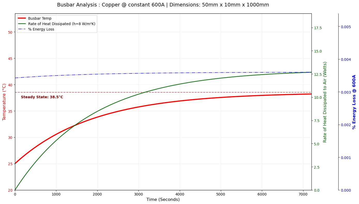
The plot shows three key metrics over a 2-hour simulation:

Red line: Busbar temperature rising to steady state
Green line: Rate of heat dissipated to air (convection)
Blue dashed: Percentage energy loss

Summary Table

Parameter	Value
Material	Copper
Dimensions (W x H x L)	50mm x 10mm x 1000mm
Mass	4.480 kg
Current	600 A
h Coefficient	8 W/m²K
Steady State Temp	38.52 °C
Final Energy Loss	0.0036 %

Code

Python Implementation (click to expand)

import numpy as np
import matplotlib.pyplot as plt
import pandas as pd

# 1. MATERIAL DATABASE
materials = {
    'Copper': {'density': 8960, 'Cp': 385, 'alpha': 0.00393, 'rho_ref': 1.68e-8},
    'Aluminum': {'density': 2700, 'Cp': 897, 'alpha': 0.0039, 'rho_ref': 2.82e-8},
    'Brass': {'density': 8500, 'Cp': 377, 'alpha': 0.0020, 'rho_ref': 7.0e-8}
}

# 2. INPUTS
CHOSEN_MATERIAL = 'Copper'
I = 600                     # Current (A)
total_time = 7200           # 2 hours
V_load = 600                # System Voltage
h_conv = 8                  # Convection coeff (W/m^2*K)

# Realistic Dimensions (in meters)
L, w, h_dim = 1.0, 0.050, 0.010
T_amb, T_ref = 25, 20

# 3. SETUP & STEADY STATE
mat = materials[CHOSEN_MATERIAL]
A = w * h_dim
As = 2 * L * (w + h_dim)
mass = mat['density'] * (L * w * h_dim)
R_ref = mat['rho_ref'] * (L / A)

# Analytical Steady State
num = (I**2 * R_ref * (1 - mat['alpha'] * T_ref)) + (h_conv * As * T_amb)
den = (h_conv * As) - (I**2 * R_ref * mat['alpha'])
T_steady = num / den

# 4. SIMULATION ENGINE
dt = total_time / 5000
steps = int(total_time / dt)
time_axis = np.linspace(0, total_time, steps)

temp_history, q_conv_history, loss_history = np.zeros(steps), np.zeros(steps), np.zeros(steps)
T_current = T_amb

for i in range(steps):
    R_t = R_ref * (1 + mat['alpha'] * (T_current - T_ref))
    Q_gen = (I**2) * R_t
    Q_conv = h_conv * As * (T_current - T_amb)

    P_total = (I * V_load) + Q_gen
    energy_loss_pct = (Q_gen / P_total) * 100

    dT_dt = (Q_gen - Q_conv) / (mass * mat['Cp'])
    T_current += dT_dt * dt

    temp_history[i], q_conv_history[i], loss_history[i] = T_current, Q_conv, energy_loss_pct

# 5. VISUALIZATION
fig, ax1 = plt.subplots(figsize=(14, 8))

ax1.plot(time_axis, temp_history, color='red', linewidth=3, label='Busbar Temp')
ax1.axhline(y=T_steady, color='darkred', linestyle='--', alpha=0.6)
ax1.set_xlabel('Time (Seconds)')
ax1.set_ylabel('Temperature (°C)', color='red')

ax2 = ax1.twinx()
ax2.plot(time_axis, q_conv_history, color='darkgreen', linewidth=2,
         label=f'Heat Dissipated (h={h_conv} W/m²K)')
ax2.set_ylabel('Heat Dissipated (Watts)', color='darkgreen')

ax3 = ax1.twinx()
ax3.spines['right'].set_position(('outward', 75))
ax3.plot(time_axis, loss_history, color='blue', linestyle='-.', label='% Energy Loss')
ax3.set_ylabel(f'% Energy Loss @ {I}A', color='blue')

plt.title(f'Busbar Analysis: {CHOSEN_MATERIAL} @ {I}A')
plt.show()

To experiment with different materials, currents, or dimensions, open the notebook in Google Colab using the button at the top.